ENGINEERING SOFTWARE / STRUCTURAL ANALYSIS
HFEA: a 3D structural workbench for humanitarian infrastructure
I built a browser workbench that makes structural calculations visible, reviewable and explicit about their limits.
- Seven
- worked examples
- 160
- baseline automated checks
- 153,000
- free nodes in the large case
- CalculiX
- numerical solver
01 / THE PROBLEM
A useful check must explain its assumptions.
I started HFEA with a practical question: how could an aid or community engineer explore a tank, shelter wall or canopy without a large desktop analysis package? A laptop with modest graphics should be enough to inspect a model. The harder requirement is honesty. An attractive stress plot is of little use if the loads, supports or material assumptions are hidden.
I designed the workbench for early structural checks and engineering discussion. I wanted someone opening my portfolio to follow a complete example, understand what was calculated and take away a readable report. I have not validated the tool through field deployment. It is an engineering prototype with a defined, tested scope, rather than a claim that software can replace structural judgement.
02 / WHAT I BUILT
A small browser client. A separate solver.
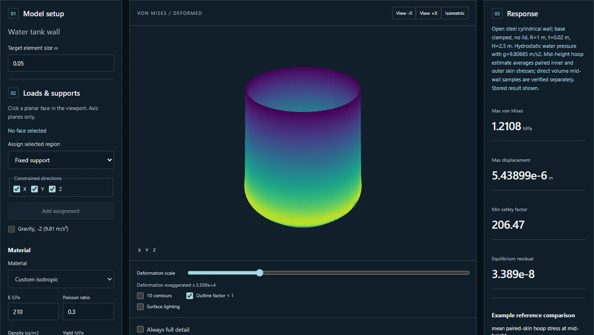
The browser handles model preparation and inspection. CalculiX performs the finite element calculation in a separate Python service. I send the outer surface, displacement and stress fields back for display instead of making the browser carry the full volume mesh. This keeps the graphics workload separate from the numerical solve and helps modest hardware remain useful.
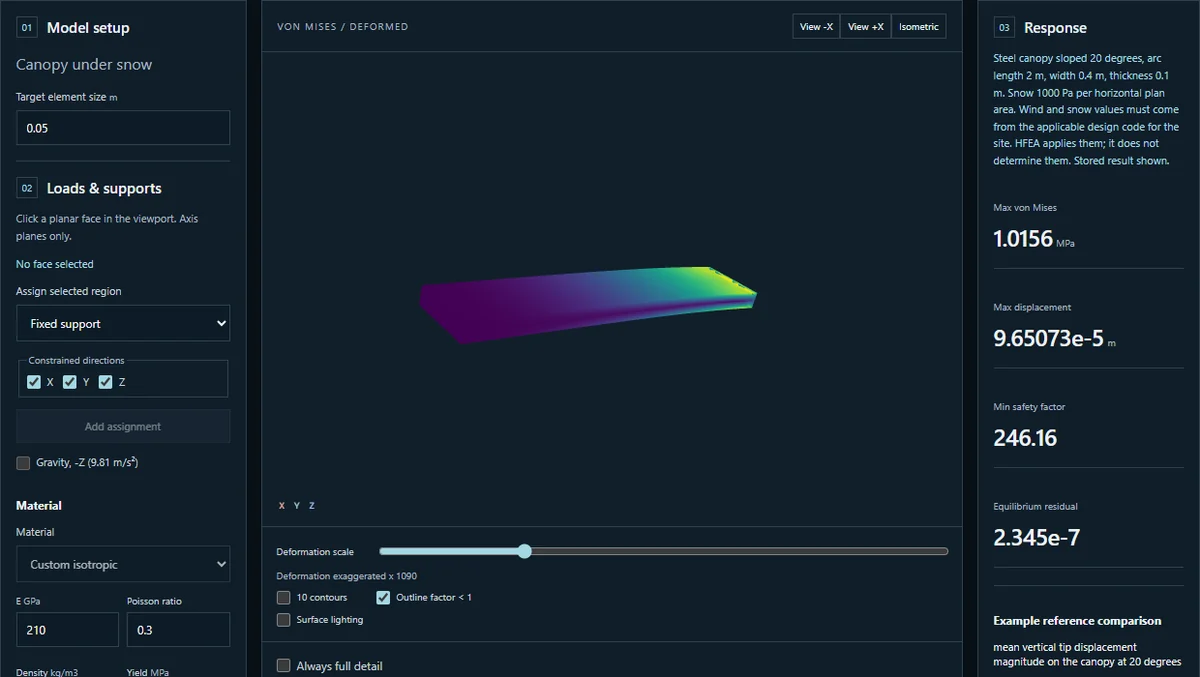
The workflow accepts an STL surface or a structured job file. Imported surfaces are meshed into tetrahedral volume elements. Users select material properties, supports and loads, then review those inputs before confirming a solve. The supported loads include water pressure varying with depth, wind pressure and snow defined over horizontal plan area. Site design values must come from the applicable engineering rules; HFEA does not choose them.
The public workbench opens seven stored examples without using the live solver. Invited users can submit models with an access token. I keep that entry masked and out of persistent browser storage. The hosted service applies individual request quotas and rate limits, alongside a shared daily limit. For the hosted deployment I worked to a USD 5 spending limit. Quotas constrain usage rather than measuring currency costs.
03 / THE EVIDENCE
Verification before presentation.
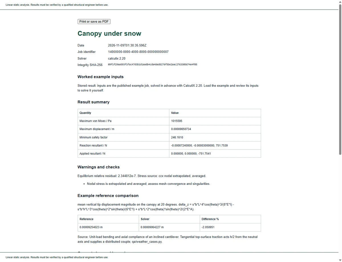
I compare the solver with independent reference solutions, including axial extension, beam deflection and thick cylinder behaviour. Those analytical benchmark gates check quantities and tolerances, not whether a picture looks plausible. I also check force equilibrium, input errors, material handling and the data sent to the viewer. The baseline solver revision completed 160 automated checks, with browser and performance gates alongside them.
I run the full reference suite in a pinned image containing Python 3.11 and CalculiX 2.20. Fixing those versions makes a test result easier to reproduce and keeps a version difference from being mistaken for a physics change. The large solve runs with four CPUs and an 8 GiB memory limit. Browser frame timing remains dependent on the graphics environment, so I report software rendering measurements separately.
| Case | Mesh or workload | Recorded time |
|---|---|---|
| Axial bar | 288 volume elements | 0.12 s solver wall time |
| Water tank wall | 24,576 volume elements | 18.62 s solver wall time |
| Canopy under snow | 1,920 volume elements | 0.58 s solver wall time |
| Large cantilever | 153,000 free nodes | 101.02 s total wall time |
The large case used 3.40 GB peak container memory in that run. A later reference run completed in 83.46 seconds using 3.33 GB. These are measured results from particular machines and runs, not service guarantees. The example timings above are stored solver measurements; they exclude download and display time. Opening a public example reads that stored result rather than repeating its calculation.
04 / AN IMPORTANT FAILURE MODE
Geometry changes must be visible.
A live trial with nine STL files produced seven solved results and two explicit meshing refusals. The successful files ranged from 8,154 to 30,879 nodes. The two refused surfaces could not be converted into tetrahedral volumes. I count those refusals as useful information, not successful analysis. The trial also exposed a more subtle problem: the mesher could repair a deliberately damaged surface without telling the person who uploaded it.
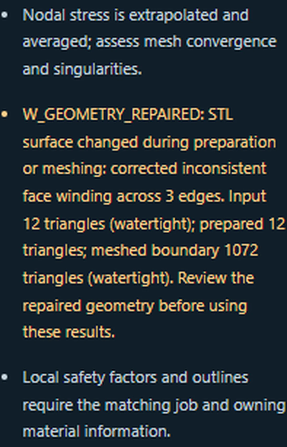
I added a geometry audit and an amber repair warning. It compares triangle counts, surface closure and changes during preparation or meshing. A flipped face now produces a visible notice explaining the winding correction and showing the input, prepared and meshed triangle counts. The full message stays in the analysis notes and printable report. A result can therefore be numerically available while still requiring a careful geometry review.
05 / ENGINEERING DECISIONS
Choose a scope that can be checked.
I kept the analysis linear and static. That makes the supported behaviour easier to verify, but it leaves out effects such as plastic deformation, buckling and dynamic response. I also chose explicit input review over immediate solving. After watching a visitor journey, I numbered the review and confirmation steps, cleared stale example labels after uploads and brought warnings closer to the viewer. These details help people understand which model they are actually assessing.
My next step is a physical cantilever rig with a load cell and strain gauges, comparing measured strain and displacement with predictions and their uncertainty. The rig software is prepared; physical correlation is still future work. I would also extend element support as new use cases justify it, with a reference problem and acceptance tests for each addition.